Let’s take a deep dive into reinforcement learning. In this article, we will tackle a concrete problem 使用TensorFlow等现代库, TensorBoard, Keras, and OpenAI gym. 您将看到如何实现称为深度Q学习的基本算法之一，以了解其内部工作原理. Regarding the hardware, 整个代码将在典型的PC上工作，并使用所有找到的CPU内核(这是由TensorFlow处理的).

The problem is called Mountain Car: A car is on a one-dimensional track, 位于两座山之间. The goal is to drive up the mountain on the right (reaching the flag). 然而，这辆车的发动机不够强大，无法一次翻过这座山. 因此，成功的唯一途径是来回驾驶，以建立动力.

选择这个问题是因为它很简单，可以在几分钟内在单个CPU核心上找到强化学习的解决方案. However, it is complex enough to be a good representative.

首先，我将简要总结一下强化学习的一般功能. Then, we will cover basic terms and express our problem with them. After that, 我将描述深度$Q$学习算法，我们将实现它来解决问题.

强化学习基础

Reinforcement learning in the simplest words is learning by trial and error. The main character is called an “agent,” which would be a car in our problem. 代理在一个环境中做出一个动作，并得到一个新的观察结果和该动作的奖励. Actions leading to bigger rewards are reinforced, hence the name. As with many other things in computer science, this one was also inspired by observing live creatures.

agent与环境的交互总结如下图所示:

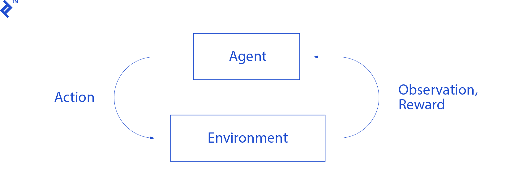
The agent gets an observation and reward for the performed action. Then it makes another action and takes step two. 环境现在返回一个(可能)略有不同的观察和奖励. 这一直持续到到达终端状态，通过向代理发送“done”发出信号. The whole sequence of observations > actions > next_observations > rewards 被称为一个插曲(或轨迹).

Going back to our Mountain Car: our car is an agent. The environment is a black-box world of one-dimensional mountains. 汽车的动作归结为只有一个数字:如果是正数，发动机将汽车推向右侧. 如果是负的，它把车推到左边. 代理通过观察感知环境:汽车的X位置和速度. If we want our car to drive on top of the mountain, 我们用一种方便的方式来定义奖励:agent每走一步没有达到目标，其奖励就减去-1. 当它达到目标时，这一集就结束了. 所以，实际上，行为人因为没有处于我们希望的位置而受到惩罚. 他越快到达，对他越好. 代理的目标是最大化总奖励，即一集的奖励总和. 如果它在e之后到达期望的点.g., 110 steps, 它的总收益是-110, which would be a great result for Mountain Car, 因为如果没有达到目标, 然后惩罚它走200步(因此, a return of -200).

这就是整个问题的表述. Now, 我们可以把它交给算法, 它们已经足够强大，可以在几分钟内解决这些问题(如果调整得当)。. It’s worth noting that we don’t tell the agent how to achieve the goal. We don’t even provide any hints (heuristics). The agent will find a way (a policy) to win on its own.

搭建环境

First, copy the whole tutorial code onto your disk:

git clone http://github.com/AdamStelmaszczyk/rl-tutorial
cd rl-tutorial

Now, we need to install Python packages that we will use. To not install them in your userspace (and risk collisions), we will make it clean and install them in the conda environment. If you do not have conda installed, please follow http://conda.io/docs/user-guide/install/index.html.

为了创造我们的conda环境:

Conda create -n tutorial python=3.6.5 -y

To activate it:

source activate tutorial

You should see (tutorial) 在shell中的提示符附近. It means that a conda environment with the name “tutorial” is active. 从现在开始，所有命令都应该在该conda环境中执行.

Now, we can install all dependencies in our hermetic conda environment:

PIP安装-r要求.txt

We are done with the installation, so let’s run some code. We don’t need to implement the Mountain Car environment ourselves; the OpenAI Gym library provides that implementation. 让我们看看环境中的一个随机代理(一个采取随机行动的代理):

import gym

env = gym.make('MountainCar-v0')
done = True
episode = 0
episode_return = 0.0
for episode in range(5):
   for step in range(200):
       if done:
           if episode > 0:
               print("Episode return: "， episode_return)
           obs = env.reset()
           episode += 1
           episode_return = 0.0
           env.render()
       else:
           obs = next_obs
       action = env.action_space.sample()
       Next_obs，奖励，完成，_ = env.step(action)
       episode_return += reward
       env.render()

This is see.py file; to run it, execute:

python see.py

You should see a car going randomly back and forth. Each episode will consist of 200 steps; the total return will be -200.

Now we need to replace random actions with something better. 有很多算法可以使用. 作为入门教程，我认为一种叫做深度Q学习的方法是很合适的. 理解这种方法为学习其他方法奠定了坚实的基础.

Deep $Q$-learning

The algorithm that we will use was first described in 2013 by Mnih et al. in Playing Atari with Deep Reinforcement Learning 并在两年后打磨 Human-level control through deep reinforcement learning. 许多其他工作都是建立在这些结果之上的，包括目前最先进的算法 Rainbow (2017):

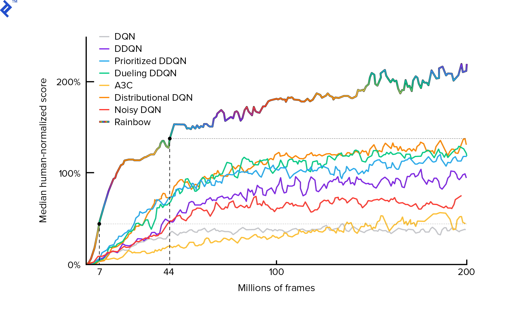
Rainbow achieves superhuman performance on many Atari 2600 games. 我们将专注于基本的DQN版本, with as small a number of additional improvements as possible, 为了保持本教程的合理大小.

A policy, typically denoted $π(s)$, 函数是否返回在给定状态下采取单个动作的概率$s$. 因此，例如，一个随机的Mountain Car策略对任何州都返回:50%左，50%右. 在游戏过程中，我们从该策略(分布)中取样以获得真实的行动.

$Q$-learning (Q为Quality)是表示$Q_π(s, a)$的动作值函数. It returns the total return from a given state $s$, choosing action $a$, 遵循一个具体的政策$π$. The total return is the sum of all rewards in one episode (trajectory).

如果我们知道最优Q函数，记作Q^*，我们就可以很容易地解决这个博弈. We would just follow the actions with the highest value of $Q^*$, i.e.，预期回报最高. This guarantees that we will reach the highest possible return.

然而，我们常常不知道$Q^*$. 在这种情况下，我们可以从与环境的相互作用中近似或“学习”. 这是名字中的“$Q$-learning”部分. 里面还有个"深"字，因为, 来近似这个函数, 我们将使用深度神经网络, 哪些是通用函数逼近器. 近似Q值的深度神经网络被命名为深度Q网络(Deep Q- networks, DQN)。. In simple environments (with the number of states fitting in memory), 我们可以用一个表代替神经网络来表示Q函数, in which instance it would be named “tabular $Q$-learning.”

So our goal now is to approximate the $Q^*$ function. 我们将使用Bellman方程:

\[Q(s, a) = r + γ \space \textrm{max}_{a'} Q(s', a')\]

$s ' $是$s$后面的州. $γ$ (gamma), typically 0.99, is a discount factor (it’s a hyperparameter). 它对未来奖励的权重较小(因为它们比我们不完美的即时奖励更不确定)。. The Bellman equation is central to deep $Q$-learning. 它表示给定状态和行为的Q值是在采取行动a后获得的奖励r plus the highest $Q$-value for the state we land in $s’$. The highest is in a sense that we are choosing an action $a’$, which leads to the highest total return from $s’$.

对于Bellman方程，我们可以使用监督学习来近似Q^*$. 函数Q将用神经网络权重表示(参数化)，表示为$θ$ (θ). 一个简单的实现将把一个状态和一个动作作为网络的输入和输出q值. 低效率是，如果我们想知道给定状态下所有动作的Q值, we need to call $Q$ as many times as there are actions. 有一种更好的方法:只将状态作为所有可能动作的输入和输出Q值. 多亏了这一点，我们可以在一次向前传递中获得所有动作的Q值.

We start training the $Q$ network with random weights. From the environment, we obtain many transitions (or “experiences”). 这些是(状态，行动，下一状态，奖励)的元组，或者，简而言之，($s$， $a$， $s ' $， $r$). We store thousands of them in a ring buffer called “experience replay.” Then, 我们从这个缓冲中抽取经验，希望Bellman方程对它们成立. We could have skipped the buffer and applied experiences one by one (this is called “online” or “on-policy”); the problem is that subsequent experiences are highly correlated with each other and DQN trains poorly when this occurs. That’s why the experience replay was introduced (an “offline,” “off-policy” approach) to break out this data correlation. The code of our simplest ring buffer implementation can be found in the replay_buffer.py 文件，我鼓励你阅读.

In the beginning, 因为我们的神经网络权重是随机的, Bellman方程左边的值会离右边很远. The squared difference will be our loss function. 我们将通过改变神经网络的权值$θ$来最小化损失函数. 我们把损失函数写下来

\[L(θ) = [Q(s, a) - r - γ \space \textrm{max}_{a'}Q(s', a')]^2\]

这是一个改写的贝尔曼方程. 假设我们从《欧博体育app下载》体验回放中采样了一次体验($s$，左，$s$， -1). 我们用状态$s$在$Q$网络中做一个前向传递，对于左动作，它给我们-120, for example. 因此，$Q(s， \textrm{left}) = -120$. Then we feed $s’$ to the network, which gives us, e.g.左边-130，右边-122. 因此，显然$s ' $的最佳操作是正确的，因此$\textrm{max}_{a '}Q(s '， a ') = -122$. We know $r$, this is the real reward, which was -1. 所以我们的$Q$-network预测有一点错误，因为$L(θ) = [-120 -1 + 0].99 ⋅ 122]^2 = (-0.22^2) = 0.0484$. So we backward propagate the error and correct the weights $θ$ slightly. 如果我们为同样的经历再次计算损失，它现在会更低.

One important observation before we go to code. 让我们注意到，为了更新DQN，我们将对DQN本身进行两次前向传递. 这通常会导致不稳定的学习. 为了缓解这种情况，对于下一个状态$Q$预测，我们不使用相同的DQN. We use an older version of it, which in the code is called target_model (instead of model, being the main DQN). 多亏了这一点，我们有了一个稳定的目标. We update target_model by setting it to model weights every 1000 steps. But model updates every step.

Let’s look at the code creating the DQN model:

def create_model(env):
   n_actions = env.action_space.n
   obs_shape = env.observation_space.shape
   Observations_input = keras.layers.输入(obs_shape, name = ' observations_input ')
   action_mask = keras.layers.输入((n_actions)、name = ' action_mask ')
   hidden = keras.layers.Dense(32, activation='relu')(observations_input)
   hidden_2 = keras.layers.密度(32,激活= relu)(隐藏)
   output = keras.layers.密度(n_actions) (hidden_2)
   filtered_output = keras.layers.乘([输出,action_mask])
   model = keras.models.Model([observations_input, action_mask], filtered_output)
   optimizer = keras.optimizers.亚当(lr = LEARNING_RATE clipnorm = 1.0)
   model.compile(optimizer, loss='mean_squared_error')
   return model

First, 该函数从给定的OpenAI Gym环境中获取动作和观察空间的维度. It is necessary to know, for example, how many outputs our network will have. 它必须等于动作的数量. 动作是一个热编码:

Def one_hot_encode(n, action):
   one_hot = np.zeros(n)
   one_hot[int(action)] = 1
   return one_hot

So (e.g.) left will be [1, 0] and right will be [0, 1].

We can see the observations are passed as input. We also pass action_mask as a second input. Why? 在计算$Q(s,a)$时，我们只需要知道一个给定动作的$Q$值，而不是所有动作的$Q$值. action_mask contains 1 for the actions that we want to pass to the DQN output. If action_mask 为0，那么相应的$Q$值将在输出上归零. The filtered_output layer is doing that. 如果我们想要所有的$Q$-值(用于最大计算)，我们可以传递所有的值.

The code uses keras.layers.Dense 定义一个完全连接的层. Keras is a Python library for higher-level abstraction on top of TensorFlow. Under the hood, Keras创建一个TensorFlow图, with biases, 适当的权重初始化, 还有其他低级别的东西. 我们可以只使用原始的TensorFlow来定义图形，但它不会是一行代码.

因此，观察结果通过ReLU(整流线性单元)激活传递到第一个隐藏层. ReLU(x) 只是一个$\textrm{max}(0, x)$函数. That layer is fully connected with a second identical one, hidden_2. The output layer brings down the number of neurons to the number of actions. In the end, we have filtered_output，它只是将输出乘以 action_mask.

为了找到$θ$权重，我们将使用一个具有均方误差损失的名为“Adam”的优化器.

有了一个模型，我们可以用它来预测给定状态观测值的Q值:

Def predict(env, model, observations):
   action_mask = np.((len(观察),env.action_space.n))
   return model.预测(x =[观察,action_mask])

We want $Q$-values for all the actions, thus action_mask is a vector of ones.

要做实际的训练，我们将使用 fit_batch():

def fit_batch(env, model, target_model, batch):
   observations, actions, rewards, next_observations, dones = batch
   #预测下一个状态的Q值. 传递一个作为动作掩码.
   next_q_values = predict(env, target_model, next_observations)
   # The Q values of terminal states is 0 by definition.
   next_q_values[dones] = 0.0
   #每个开始状态的Q值等于奖励+伽马*下一个状态的最大Q值
   q_values = rewards + DISCOUNT_FACTOR_GAMMA * np.马克斯(next_q_values轴= 1)
   one_hot_actions = np.数组([one_hot_encode (env.action_space.(动作中的动作)
   history = model.fit(
       x =[观察,one_hot_actions],
       y=one_hot_actions * q_values[:， None]，
       batch_size=BATCH_SIZE,
       verbose=0,
   )
   return history.history['loss'][0]

Batch contains BATCH_SIZE experiences. next_q_values is $Q(s, a)$. q_values is $r + γ \space \textrm{max}_{a’}Q(s’, a’)$ from the Bellman equation. Actions we took are one hot encoded and passed as action_mask 调用时的输入 model.fit(). $y$ is a common letter for a “target” in supervised learning. Here we are passing the q_values. I do q_values[:. None] 来增加数组的维度，因为它必须对应于的维度 one_hot_actions array. This is called slice notation if you would like to read more about it.

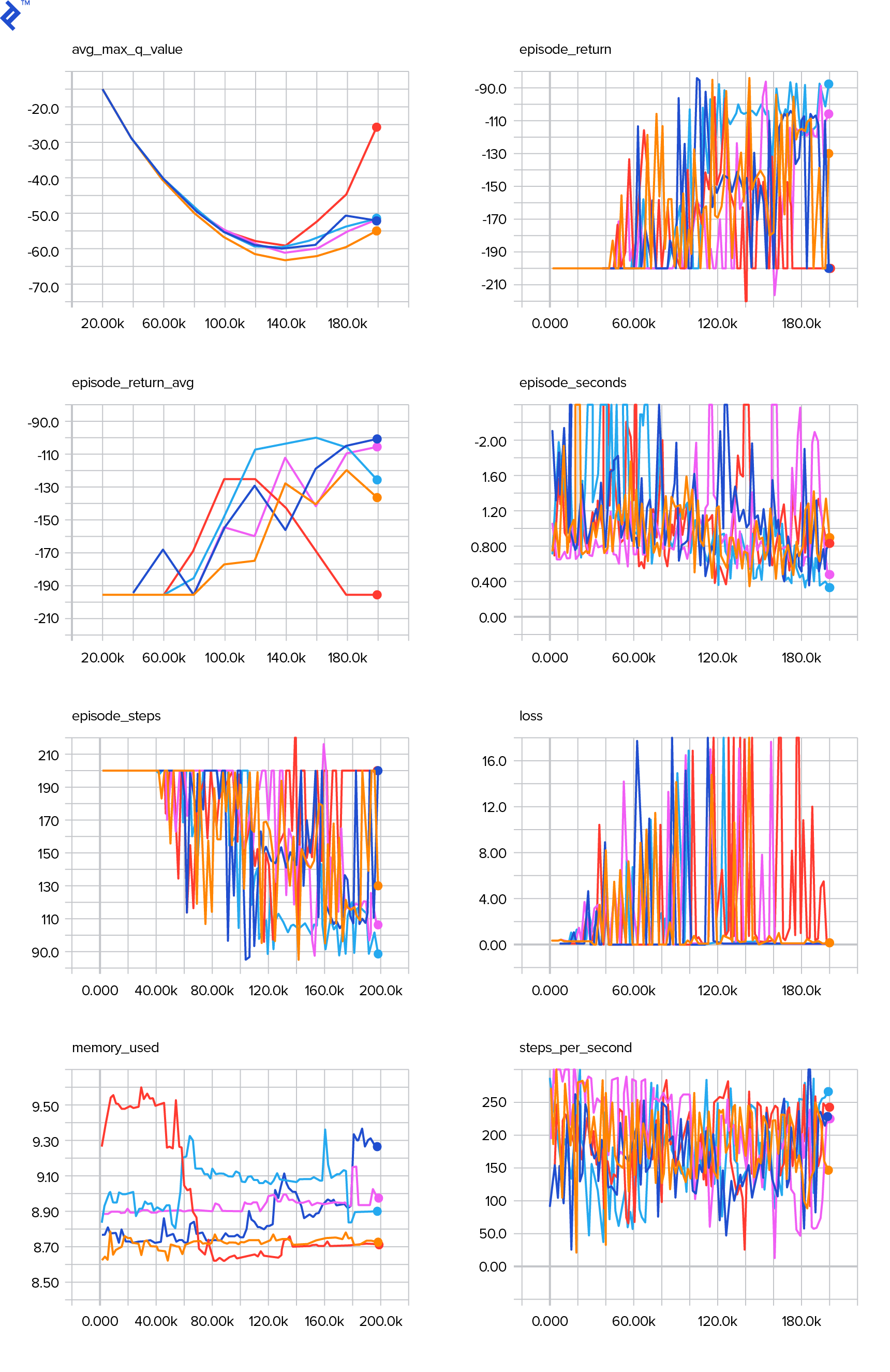
我们返回损失以将其保存在TensorBoard日志文件中，稍后进行可视化. 还有很多其他的事情我们要监控:我们每秒走多少步, total RAM usage, 平均每集的收益是多少, etc. Let’s see those plots.

Running

To visualize the TensorBoard log file, we first need to have one. 让我们来运行这个训练:

python run.py

This will first print the summary of our model. 然后，它将用当前日期创建一个日志目录，并开始训练. Every 2000 steps, a logline will be printed similar to this:

第10集步骤200/2001输0.3346639 return -200.0 in 1.02s 195.7 steps/s 9.0/15.6 GB RAM

Every 20,000, we will evaluate our model on 10,000 steps:

Evaluation
100%|█████████████████████████████████████████████████████████████████████████████████| 10000/10000 [00:07<00:00, 1254.40it/s]
episode 677 step 120000 episode_return_avg -136.750 avg_max_q_value -56.004

在677集和12万步之后，平均集回报从-200提高到-136.75! It’s definitely learning. What avg_max_q_value is I’m leaving as a good exercise to the reader. But it’s a very useful statistic to look at during training.

20万步之后，我们的训练就完成了. On my four-core CPU, it takes about 20 minutes. We can look inside the date-log directory, e.g., 06-07-18-39-log. 将有四个模型文件 .h5 extension. This is a snapshot of TensorFlow graph weights, we save them every 50,000 steps to later have a look at the policy we learned. To view it:

python run.py --model 06-08-18-42-log/06-08-18-42-200000.h5 --view

查看其他可能的标志: python run.py --help.

Now, the car is doing a much better job of reaching the desired goal. In the date-log 目录，也有 events.out.* file. This is the file where TensorBoard stores its data. 我们用最简单的方式写信给它 TensorBoardLogger defined in loggers.py. To view the events file, we need to run the local TensorBoard server:

tensorboard --logdir=.

--logdir just points to the directory in which there are date-log directories, in our case, 这将是当前目录, so .. TensorBoard prints the URL at which it is listening. If you open up http://127.0.0.1:6006, you should see eight plots similar to these:

Wrapping Up

train() does all the training. We first create the model and replay the buffer. 然后，在一个非常类似的循环中 see.py, we interact with the environment and store experiences in the buffer. What’s important is that we follow an epsilon-greedy policy. We could always choose the best action according to the $Q$-function; however, 这会阻碍探索, 这会损害整体表现. 因此，为了执行具有epsilon概率的探索，我们执行随机操作:

Def greedy_action(env, model, observation):
   next_q_values = predict(env, model, observations=[observation])
   return np.argmax(next_q_values)


def epsilon_greedy_action(env, model, observation, epsilon):
   if random.random() < epsilon:
       action = env.action_space.sample()
   else:
       action = greedy_action(env, model, observation)
   return action

Epsilon was set to 1%. After 2000 experiences, the replay fills up enough to start the training. We do it by calling fit_batch() with a random batch of experiences sampled from the replay buffer:

batch = replay.sample(BATCH_SIZE)
loss = fit_batch(env, model, target_model, batch)

Every 20,000 steps, we evaluate and log the results (evaluation is with epsilon = 0(完全贪婪的政策):

if step >= TRAIN_START and step % EVAL_EVERY == 0:
   Episode_return_avg = evaluate(env, model)
   q_values = predict(env, model, q_validation_observations)
   max_q_values = np.max(q_values, axis=1)
   avg_max_q_value = np.mean(max_q_values)
   print(
       "episode {} "
       "step {} "
       "episode_return_avg {:.3f} "
       "avg_max_q_value {:.3f}".format(
           episode,
           step,
           episode_return_avg,
           avg_max_q_value,
       ))
   logger.log_scalar('episode_return_avg', episode_return_avg, step)
   logger.log_scalar('avg_max_q_value', avg_max_q_value, step)

整个代码大约有300行，并且 run.py contains about 250 of the most important ones.

One can notice there are a lot hyperparameters:

Discount_factor_gamma = 0.99
LEARNING_RATE = 0.001
BATCH_SIZE = 64
Target_update_every = 1000
TRAIN_START = 2000
Replay_buffer_size = 50000
MAX_STEPS = 200000
LOG_EVERY = 2000
SNAPSHOT_EVERY = 50000
EVAL_EVERY = 20000
EVAL_STEPS = 10000
EVAL_EPSILON = 0
TRAIN_EPSILON = 0.01
Q_validation_size = 10000

这还不是全部. 还有一个网络架构——我们使用了两个隐藏层，包含32个神经元, ReLU activations, and Adam optimizer, 但是还有很多其他的选择. Even small changes can have a huge impact on training. A lot of time can be spent tuning hyperparameters. In a recent OpenAI competition, a second-place contestant found out it is possible to almost double 彩虹在超参数调优后的分数. Naturally, one has to remember that it’s easy to overfit. 目前，强化算法正在努力将知识转移到类似的环境中. Our Mountain Car doesn’t generalize to all types of mountains right now. 你可以修改OpenAI Gym环境，看看agent能泛化到什么程度.

Another exercise will be to find a better set of hyperparameters than mine. It’s definitely possible. 然而，一次训练并不足以判断你的改变是否是一种进步. There usually is a be a big difference between training runs; the variance is big. You would need many runs to determine that something is better. If you would like to read more about such important topic as reproducibility, I encourage you to read 深度强化学习很重要. 而不是手工调弦, 如果我们愿意在这个问题上花费更多的计算能力，我们可以在某种程度上自动化这个过程. 一种简单的方法是为一些超参数准备一个有希望的值范围，然后运行网格搜索(检查它们的组合)。, 培训并行进行. 并行化本身就是一个大话题，因为它对高性能至关重要.

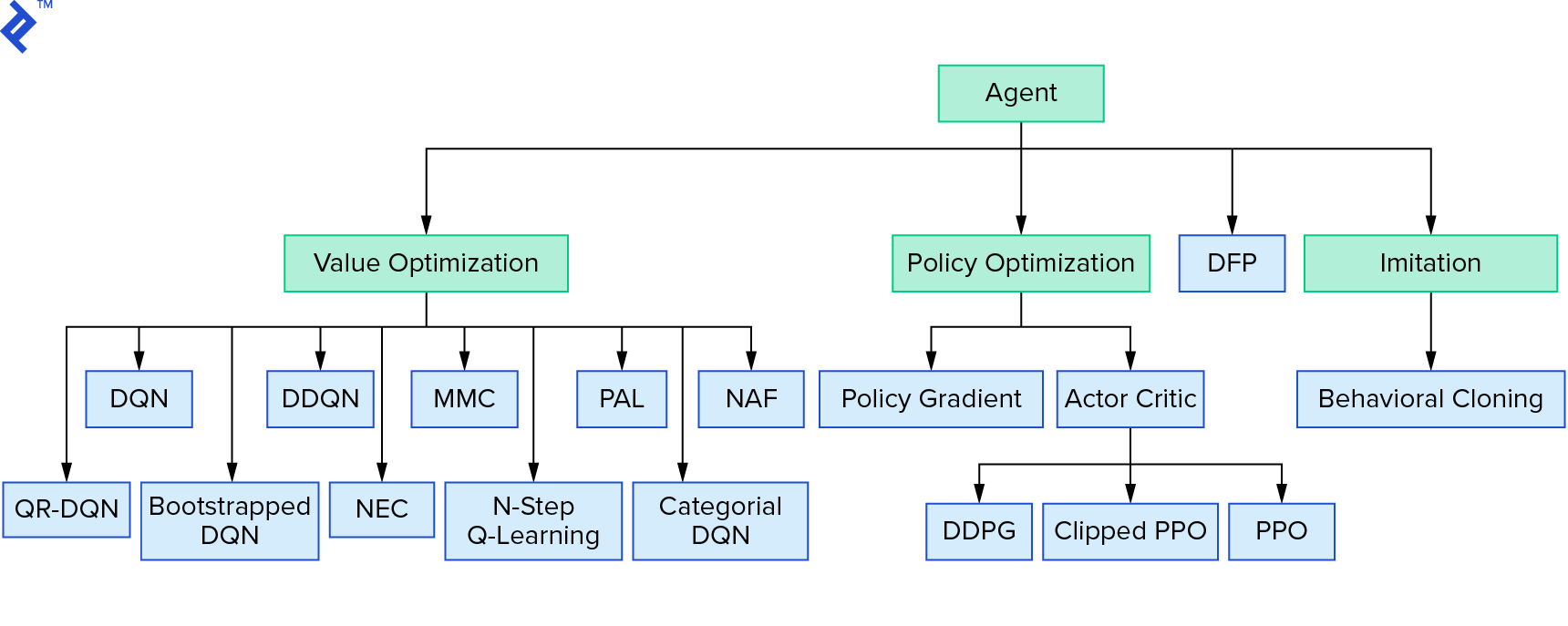
深度Q学习代表了一大类使用值迭代的强化学习算法. 我们试着近似Q函数，大多数时候我们只是贪心地使用它. There is another family that uses policy iteration. 他们的重点不是逼近Q函数，而是直接找到最优策略π^*$. 为了了解值迭代在强化学习算法中的位置:

Your thoughts could be that deep reinforcement learning looks brittle. You will be right; there are many problems. You can refer to 深度强化学习还不起作用 and Reinforcement Learning never worked, and ‘deep’ only helped a bit.

本教程到此结束. We implemented our own basic DQN for learning purposes. Very similar code can be used to achieve good performance in some of the Atari games. 在实际应用程序中，通常采用经过测试的高性能实现，例如.g., one from OpenAI baselines. 如果你想看看在更复杂的环境中应用深度强化学习会面临什么样的挑战, you can read 我们的NIPS 2017:学习跑步方法. 如果你想在一个有趣的竞争环境中学习更多，看看 NIPS 2018 Competitions or crowdai.org.

如果你正在成为一名 machine learning 专家，想加深你在监督学习方面的知识，请查看 Machine Learning Video Analysis: Identifying Fish 为了一个有趣的识别鱼的实验.